Bayesian state-space and hierarchical modelling of bank deposit rates
Banks live and die by their cheapest source of funding: customer deposits in current and savings accounts. Unlike a fixed-term bond, these non-maturing deposits (NMDs) have no contractual maturity, i.e., depositors can walk at any time, and the bank sets the rate administratively rather than via a contract. That makes them hard to model and easy to get wrong: under-estimate how quickly depositors will flee when rates rise, and your interest-rate-risk report is fiction.
This post walks through a model I built for these dynamics in Python and PyMC, end-to-end on real ECB AAA yield curve data from 2014 to 2024.
👉 Overview notebook (HTML render):
https://thomasmartins.github.io/nmd-rates-pymc/notebooks/00_main.html
1. Why this is a hard modelling problem
Three things make NMD rates uncooperative:
- Pass-through is administrative and lagged. When the central bank hikes, you don’t see deposit rates move the next morning. Rate cards are adjusted periodically, and even then only by some fraction of the market move.
- Pass-through is heterogeneous across customer segments. Corporate treasuries shop their cash aggressively and demand market-aligned rates. Retail current-account holders, in many cases, never look. A single pass-through coefficient averages across these and is wrong for everyone.
- The 2015–2024 ECB data has an obvious structural break. During the negative-rate era (2015–2021) banks barely passed cuts on at all, because the zero lower bound made further cuts uneconomic. Then in 2022 ECB hikes started and pass-through suddenly mattered again. Fitting a single static model across this period gives you a useless average of two distinct regimes.
The model has three stages, each addressing one of these problems.
2. Pipeline overview
        Diebold-Li               Hierarchical ECM            Hierarchical AR(1)
ECB     state-space      latent  + Markov regimes  deposit  + spread          volumes,
yields ───────────────►  factors ────────────────► rates    sensitivity ────► NII
        Kalman + NUTS    L, S, C Hamilton filter            soft regime
                                                            covariate
Each stage uses a different piece of Bayesian machinery. I walk through them in turn below.
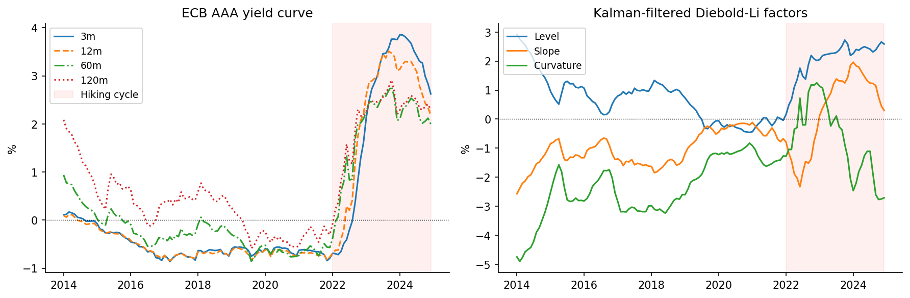
3. Stage 1: Yield curve as a Bayesian state-space model
The first job is to turn 132 months of an 8-maturity yield curve into three interpretable factors: level, slope and curvature. The Nelson–Siegel parameterisation does this with a fixed loading matrix:
\[y_t(\tau) \;=\; L_t \;+\; S_t\cdot\frac{1-e^{-\lambda\tau}}{\lambda\tau} \;+\; C_t\cdot\!\left(\frac{1-e^{-\lambda\tau}}{\lambda\tau}-e^{-\lambda\tau}\right).\]Diebold and Li (2006) made this dynamic by treating the three factors as latent states with VAR(1) dynamics, giving a textbook linear-Gaussian state-space model. The natural estimator is the Kalman filter, which returns the exact marginal likelihood
\[\log p(\mathbf{Y}\mid\boldsymbol\theta) \;=\; \sum_{t=1}^{T}\!\left[ -\tfrac{J}{2}\log 2\pi -\tfrac{1}{2}\log|\mathbf S_t| -\tfrac{1}{2}\mathbf v_t^\top \mathbf S_t^{-1}\mathbf v_t \right].\]For classical statistics (frequentist) that’s the end of it: maximise the likelihood, report standard errors. The Bayesian version is more interesting: wrap the whole Kalman recursion in pytensor.scan (PyMC’s loop primitive) and let NUTS auto-differentiate through it, sampling the full posterior over \((\boldsymbol\mu, \boldsymbol\Phi, \mathbf Q, \sigma_{\text{obs}})\).
What you get out is not just point estimates but a joint posterior over all factor dynamics, which is exactly what the downstream models need. The yield curve fit RMSE across 132 months × 8 maturities is 0.066 pp.
4. Stage 2: Hierarchical ECM with Markov regime switching
Now the harder stage. The naive thing is to regress deposit rates on the filtered factors:
\[r_{s,t} \;=\; \alpha_s + \beta^L_s L_t + \beta^S_s S_t + \beta^C_s C_t + \varepsilon_{s,t}.\]This is wrong for two reasons we already saw: it doesn’t allow lagged adjustment, and it can’t represent the structural break. We fix both at once.
Sluggish adjustment: an error correction model
Define a long-run equilibrium rate \(r^*_{s,t-1}\) (the static regression above), and let observed rates close the gap to it at a segment-specific speed \(\gamma_s\):
\[\Delta r_{s,t} \;=\; \gamma_s\,(r_{s,t-1} - r^*_{s,t-1}) + \varepsilon_{s,t}, \qquad \gamma_s \in (-1, 0).\]The half-life of adjustment is \(-\log 2 / \log(1+\gamma_s)\) months. The estimated half-lives range from 0.9 months for corporates (almost instant repricing) to 3.0 months for retail current accounts (slow).
The regime-switching part
To handle the structural break, \(r^*\) becomes a function of a hidden binary regime \(z_t \in \{0, 1\}\):
\[r^*_{s,t-1}(z_t) \;=\; \alpha_s + \beta^{L,(z_t)}_s\,L_{t-1} + \beta^{S,(z_t)}_s\,S_{t-1} + \beta^{C}_s\,C_{t-1}.\]with \(z_t\) following a first-order Markov chain. Since \(z_t\) is unobserved, we can’t condition on it, thus we have to marginalise it out. That’s the Hamilton (1989) filter: the discrete-state analogue of the Kalman filter.
The Hamilton filter does the same predict–update dance as Kalman, but with categorical states. The predict step is a matrix–vector multiply \(\xi_{t\mid t-1} = P^\top \xi_{t-1\mid t-1}\); the update step is Bayes’ rule applied element-wise. The denominator of the update is the one-step-ahead likelihood contribution: summing the log of that over \(t\) gives the marginal log-likelihood we hand to NUTS.
Just like the Kalman filter in stage 1, the Hamilton filter lives inside a pytensor.scan loop, so NUTS differentiates through it and samples the full joint posterior over regime probabilities, the transition matrix, and the segment-level betas simultaneously. There is no separate EM step or post-hoc regime classification.
Identification
The two regimes are otherwise interchangeable (a label-swap symmetry). Standard fix: impose a sign constraint. We model the regime-1 pass-through as \(\mu^{(1)}_{\beta L} = \mu^{(0)}_{\beta L} + \delta\) with \(\delta\sim\text{HalfNormal}(0.30)\), forcing \(\delta > 0\). Regime 1 is defined as the higher-pass-through state.
Hierarchical partial pooling
The four segments each get their own parameters, but they’re drawn from common population distributions (\(\beta^{L,(k)}_s \sim \mathcal{N}(\mu^{(k)}_{\beta L},\;\sigma_{\beta L})\), etc.). This is partial pooling: noisy segment estimates get shrunk toward the population mean, while well-identified segments retain their own estimate. With only \(S=4\) segments the pooling effect is mild, but the structure naturally encodes a sensible prior: similar segments should have similar pass-through.
Non-centred parameterisation throughout, to avoid the funnel-shaped posteriors that hierarchical models produce when group variances are small.
The headline result
The filtered regime probability over time recovers the true 2022 break with 98.5% classification accuracy:
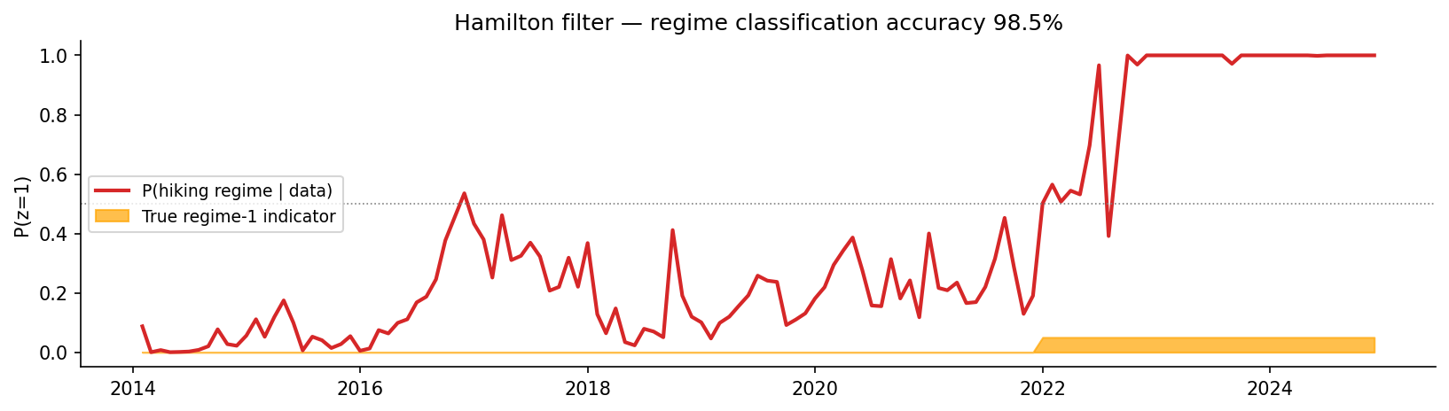
And the estimated betas pick up exactly the economic story we’d expect:
| Segment | γ (speed) | Half-life | β_L low rate | β_L hiking | Amplification |
|---|---|---|---|---|---|
| Retail Current | –0.20 | 3.0 m | 0.08 | 0.13 | 1.7× |
| Retail Savings | –0.20 | 3.0 m | 0.08 | 0.29 | 3.5× |
| SME Operational | –0.31 | 1.9 m | 0.15 | 0.43 | 2.9× |
| Corporate | –0.53 | 0.9 m | 0.19 | 0.66 | 3.4× |
In the low-rate regime pass-through is essentially zero across the board. In the hiking regime it fans out: a Retail Current account sees 13 bp of deposit-rate move per 100 bp of yield curve level shift, while a Corporate account sees 66 bp.
5. Stage 3: Volumes: hierarchical AR(1) with a soft regime covariate
Rates aren’t the full story for net interest income. When the gap between market rates and what depositors get paid widens, money walks: depositors shift to higher-yielding alternatives, and balances contract. So we need a volume model too.
Log-volumes follow a partial-adjustment AR(1) per segment, with a spread-sensitivity term:
\[\log V_{s,t} \;=\; \alpha_s + \rho_s \log V_{s,t-1} + \beta_s(p_{t-1})\,\text{spread}_{s,t-1} + \varepsilon_{s,t},\]where \(\text{spread}_{s,t} = y^{5\mathrm y}_t - r_{s,t}\) is the opportunity cost, and
\[\beta_s(p) \;=\; \beta^0_s + \Delta\beta_s\cdot p,\qquad \beta^0_s,\,\Delta\beta_s < 0.\]The interesting trick is in \(p_{t-1}\). We don’t introduce a second hidden Markov chain for the volume model. Instead, \(p_{t-1}\) is the filtered regime probability \(P(z_{t-1}=1 \mid \text{data})\) taken directly from stage 2’s Hamilton filter. The volume model uses the regime dynamics inferred by the rates model as a soft, continuous covariate. No double-counting, no separate filter, and the spread sensitivity is allowed to amplify smoothly as the regime transitions.
A technical aside: avoiding the hierarchical funnel
In hierarchical Bayesian models, the standard half-normal prior on group standard deviations has positive density at zero. With only four segments informing \(\sigma\), the posterior can collapse near zero, and that creates a textbook geometric funnel that NUTS struggles with, even with non-centred parameterisation. Initially the volume model produced 124 divergences out of 8000 draws.
The fix was to replace HalfNormal priors on the population \(\sigma\) scales with LogNormal priors, which have zero density at zero:
This pushes the prior cleanly off the funnel apex. After this and a target acceptance bump to 0.99, divergences dropped to 11 out of 16000 draws (0.07%) with \(\hat R = 1.00\) and ESS bulk > 3000 across all hyperparameters. Parameter recovery was unchanged. The issue was geometric, not informational.
What the volume model recovers
| Segment | ρ | half-life | β_V low rate | β_V hiking |
|---|---|---|---|---|
| Retail Current | 0.981 | 36 m | –0.019 | –0.046 |
| Retail Savings | 0.951 | 14 m | –0.028 | –0.069 |
| SME Operational | 0.928 | 9 m | –0.041 | –0.085 |
| Corporate | 0.895 | 6 m | –0.061 | –0.161 |
Retail balances are very persistent (ρ ≈ 0.98, half-life ~3 years). Corporate balances less so (~6 months). Spread sensitivity is uniformly negative as depositors leave when alternatives get better, and roughly 2–3× more sensitive in the hiking regime than in the low-rate regime.
6. Scenario IRRBB results
Once all three stages are estimated, we can answer the question the ALM committee actually wants answered: under a regulatory rate shock, how do deposit rates and net interest income move?
Five standard scenarios over a 12-month horizon: baseline, parallel ±200 bp, parallel –100 bp, steepener +100 bp, flattener –100 bp. Each one applies a linear ramp to the latest filtered factors and propagates the full posterior predictive through the ECM and volume models, giving median trajectories with 80% predictive intervals.
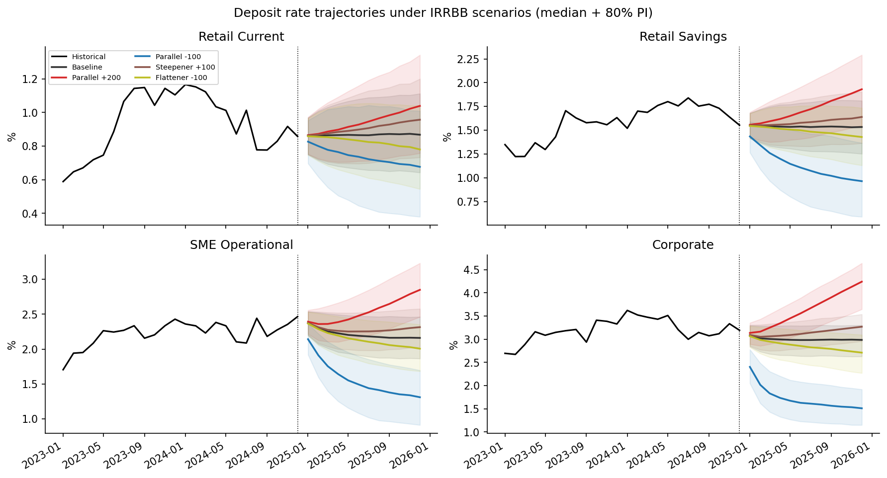
The headline number: 12-month cumulative pass-through under a +200 bp parallel shock:
| Segment | Pass-through at H=12 |
|---|---|
| Retail Current | 8.5% |
| Retail Savings | 19.7% |
| SME Operational | 34.8% |
| Corporate | 62.5% |
That ~7× fan-out from stickiest to most rate-sensitive segment is the quantity that drives both the IRRBB capital charge and the bank’s NII sensitivity to a hiking cycle. It is the output an ALM committee or a regulatory reviewer would consume directly.
7. Full notebook and repository
-
📒 Overview notebook (HTML render):
https://thomasmartins.github.io/nmd-rates-pymc/notebooks/00_main.html -
📦 GitHub repository:
https://github.com/thomasmartins/nmd-rates-pymc
Stack: PyMC 5, pytensor, NUTS via numpyro + JAX (CPU only, no GPU required), arviz, matplotlib. Python 3.11 in a conda env.
8. Final thoughts
Three things make this more than a standard hierarchical regression:
- Bayesian state-space for the yield curve. The Kalman filter wrapped in
pytensor.scangives the exact marginal likelihood and lets NUTS sample the joint posterior. Filtered factors are smoother than OLS cross-sectional estimates and carry well-calibrated uncertainty into the downstream models. - Markov regime switching with Hamilton-filter marginalisation, all inside NUTS. Joint posterior over regime probabilities, transition matrix, and segment-level betas which all together means no EM, no post-hoc classification and no two-step inference. The 2022 structural break is recovered with 98.5% classification accuracy.
- A volume model that re-uses stage 2’s regime posterior as a soft covariate. No second hidden Markov chain. The volume model inherits the regime dynamics from the rates model and amplifies its disintermediation sensitivity smoothly through the transition.
The combination of Bayesian state-space, hierarchical Markov ECM with Hamilton-filter marginalisation, and a downstream hierarchical model that re-uses upstream posteriors turns out to be a clean way to handle a problem (NMD pass-through) that is genuinely hard to model with classical tools.