Hedging Net Interest Income over time: optimal control and when reinforcement learning actually helps
A bank earns most of its money on the gap between what it charges for loans and what it pays for deposits. That spread, the net interest income (NII), is exposed to interest rates, and unlike a one-off trade, it has to be defended month after month as the yield curve moves. The treasury desk doesn’t make one hedging decision, but actually a sequence of them, each under uncertainty about where rates go next.
That structure: a state that evolves stochastically, a decision taken repeatedly, a cost accumulated over time, is exactly what dynamic control theory was built for. This post walks through treating IRRBB hedging as a control problem: estimating the state of the world with a Kalman filter on an arbitrage-free yield-curve model, computing the hedge with linear-quadratic (LQ) control, and then testing the fashionable alternative — reinforcement learning (RL), to find out when it earns its keep and when it doesn’t.
The honest one-line answer, which the rest of the post unpacks: RL beats LQ if and only if the optimal policy is nonlinear and that nonlinearity comes from the cost structure, not from fancier economics.
NII hedging is a control problem
Strip the banking book down to its rate-sensitive core. Assets of notional \(A\) reprice off a longer tenor \(\tau_A\). Liabilities of notional \(L\) reprice off a shorter tenor \(\tau_L\). Over a period \(\Delta t\), ignoring constants,
\[\text{NII}_t \;=\; A\,y_t(\tau_A)\,\Delta t \;-\; L\,y_t(\tau_L)\,\Delta t \;+\; h_t\,\big(K - y_t(\tau_L)\big)\,\Delta t .\]The first two terms are the natural book and the third is a hedge (here a pay-fixed interest-rate swaplet of notional \(h_t\) struck at \(K\)), the control we get to choose each month. A liability-sensitive bank (more funding reprices than assets) loses NII when short rates rise, so the hedge exists to flatten that exposure.
This is a textbook control setup:
- state \(x_t\): the yield curve (and the slow-moving balance sheet) at time \(t\)
- control \(u_t\): how much to change the hedge, \(h_{t+1} = h_t + u_t\)
- dynamics: the curve evolves stochastically and the the hedge inventory carries over
- cost: the variance of NII around its target, accumulated over time, plus whatever it costs to trade.
The only missing ingredient is a tractable model of the state.
The state: an arbitrage-free Nelson–Siegel curve, filtered
A full yield curve is dozens of correlated points. You don’t want dozens of state variables. The Nelson–Siegel model assumes almost all curve movement lives in three factors (level, slope, curvature) through fixed loadings
\[y_t(\tau) \;=\; X_t^{(L)} + X_t^{(S)}\,\frac{1-e^{-\lambda\tau}}{\lambda\tau} + X_t^{(C)}\!\left(\frac{1-e^{-\lambda\tau}}{\lambda\tau}-e^{-\lambda\tau}\right).\]The arbitrage-free version (AFNS, Christensen–Diebold–Rudebusch) keeps these intuitive loadings but adds a yield-adjustment term \(-C(\tau)/\tau\) so the model is internally consistent, i.e., no free lunches across maturities. That gives the best of both worlds: a three-factor state with an economic interpretation and no-arbitrage discipline.
Crucially for control, the factors aren’t observed directly: we see noisy yields at a handful of maturities. This is a linear-Gaussian state-space model, so the Kalman filter is the natural estimator: it infers the latent factors \(X_t\) from observed yields, and its likelihood, maximised over the AFNS parameters, gives the whole model by MLE. A Kalman/RTS smoother then reconstructs the factor path. The output is a clean, low-dimensional, no-arbitrage description of the state the hedger faces.
The policy: LQ / Riccati control
With a linear state and a quadratic objective (minimise the variance of NII around a target, lightly penalising how much we trade), the optimal policy is the classic linear-quadratic regulator:
\[\min_{\{u_t\}} \; \mathbb{E}\sum_t \big(\text{NII}_t - \overline{\text{NII}}\big)^2 + \lambda_u\,u_t^2 .\]Solving the discrete algebraic Riccati equation gives a linear feedback law \(u_t = -K\,[\,X_t - X_{\text{ref}};\; h_t - H_{\text{VM}}\,]\), where \(H_{\text{VM}}\) is the closed-form variance-minimising hedge ratio: the notional that makes NII as insensitive to curve moves as a single swaplet can. On the estimated AFNS model this hedge cuts NII volatility by ~60–65%, and the feedback collapses to simple proportional control toward \(H_{\text{VM}}\).
That last observation is the whole story in miniature: because NII here is contemporaneous in the curve, the best hedge is a near-constant ratio. The optimal policy is linear, and LQ delivers it exactly. There is nothing left for a cleverer method to find, a fact worth remembering when the cleverer method (reinforcement learning) shows up.
Enter reinforcement learning
Reinforcement learning attacks the same object — a sequential decision problem — but from the opposite direction. Instead of assuming a model and solving for the optimal policy, an RL agent learns a policy by trial and error against a simulator, maximising cumulative reward. Modern actor-critic algorithms like Soft Actor-Critic (SAC) handle continuous states and actions and, in principle, don’t care whether the optimal policy is linear, kinked, or wildly nonlinear.
That generality is the appeal. If the real problem has features LQ’s assumptions paper over (asymmetric (downside/CVaR) objectives, embedded optionality, hard constraints, trading frictions), then a model-free learner might find a better policy than the linear-quadratic approximation.
So I trained SAC on exactly the same hedging environment and compared it to LQ, fairly, on the same simulated paths. The result was a useful disappointment.
On the plain problem, RL does not beat LQ. It ties it, unreliably. Across a transaction-cost sweep and multiple random seeds, a naive SAC agent matched LQ’s risk reduction at best and, on some seeds, did materially worse (training variance is real; a single lucky seed is not a result). The reason is the one from the previous section: when the optimal policy is a near-constant linear hedge, LQ is already optimal, and RL’s flexibility buys nothing but variance. I also tried to manufacture an RL edge by enriching the economics (a rate-dependent balance sheet with deposit flight and mortgage prepayment) and the objective (a downside/CVaR penalty). Those change where the optimal hedge sits, but the optimal policy stays essentially linear in the observed state, so LQ tracks it and RL still can’t pull ahead.
The lesson: richer economics or objectives are not enough. To beat LQ you need the optimal policy itself to be nonlinear.
When RL wins: a fixed cost per trade
There is a clean way to force that nonlinearity, and it’s the most realistic friction of all: a fixed cost per hedging operation. Every time the desk puts on or adjusts a swap, it pays a ticket cost, independent of size. Now the objective is
\[\mathbb{E}\big[(\text{NII}-\text{target})^2\big] \;+\; \kappa_{\text{fix}}\,\mathbb{P}(\text{trade}) \;+\; \kappa_{\text{prop}}\,\mathbb{E}\lvert u\rvert .\]That single fixed term breaks LQ. A quadratic cost can’t represent “free to do nothing, expensive to do anything”, so LQ keeps rebalancing toward its moving target every single month and bleeds ticket costs. The genuinely optimal policy is qualitatively different: a no-trade band. Let the hedge drift, and only trade when it has wandered far enough from its target \(h^*_t\) to be worth a ticket:
\[\text{trade only if } \;\lvert h^*_t - h_t\rvert > b .\]This is impulse control, and the band \((s,S)\) structure is a kink no linear-quadratic feedback law can express. Here the numbers are decisive. Continuous LQ rebalancing trades every month; the optimal no-trade band trades in about 4–10% of months and costs ~50–60% less in total. Two independent methods agree on it:
- an exact impulse-control dynamic program (value iteration on the one-dimensional tracking error \(e = h - h^*\)) derives the optimal band analytically (width ≈ 11 units in the calibrated model)
- a SAC agent, told nothing about the cost structure, rediscovers it: its learned hedge is piecewise-constant, holding flat through long stretches and snapping back only occasionally, landing within a few percent of the DP optimum.
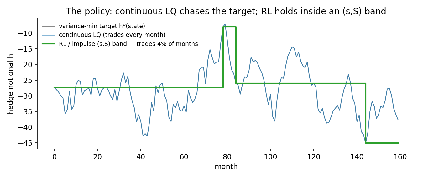
That agreement is the satisfying part. The reinforcement learner, given only states and rewards, reinvents the same nonlinear no-trade band that impulse-control theory proves is optimal, and both leave classical LQ behind. As the fixed cost rises, the band widens and the gap over LQ grows (from ~30% at a light cost to ~80% at a heavy one).
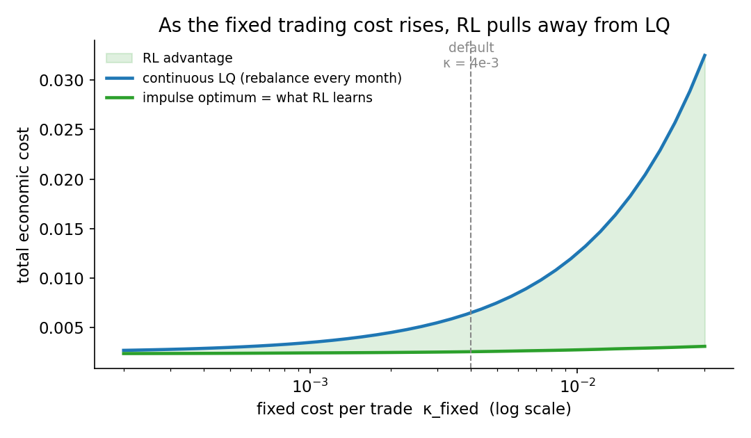
You can also watch this happen live on a slider in the interactive widget.
When to use which
Stepping back, the decision rule is clean and a little deflating for the hype:
- If the optimal policy is linear: contemporaneous exposures, smooth quadratic costs, no hard frictions, then use LQ. It’s optimal, it’s a one-line Riccati solve, it’s deterministic and reproducible, and reinforcement learning will at best tie it while adding training variance and compute.
- If the optimal policy is nonlinear: fixed/lumpy transaction costs, discrete lot sizes, hard state-dependent limits, embedded optionality that has to be dynamically delta-hedged. In this case the kink is real and LQ structurally cannot express it. That’s where RL (or, when you can discretise it, exact impulse-control DP) earns its keep.
For the IRRBB hedging problem specifically: classical control gets you ~95% of the way for free, and the remaining edge only materialises once you take trading frictions seriously. The interesting machine-learning result here isn’t “RL wins”, but it’s actually knowing precisely the condition under which it does, and being able to point at the kink that causes it.
Try it / read the details
The whole project is written up two ways: a Python research notebook (full estimation, LQ, SAC, and the impulse-control experiment) and a reactive Julia/Pluto port (the estimation and optimal-control stack, plus an exact impulse-control DP and a hand-rolled SAC), and there’s a live widget that lets you slide the trading cost and balance-sheet knobs and watch RL overtake LQ in real time.
- Full Python notebook: estimation → LQ → RL → impulse control
- Julia / Pluto notebook: estimation + optimal control, with exact DP + SAC
- Interactive widget: slide from “LQ wins” to “RL wins”
- Source:
thomasmartins/optimal-nii-hedging
Closing
Dynamic control theory and reinforcement learning are often framed as rivals, as old-school versus modern or model-based versus model-free. On a real problem they turn out to be complements with a sharp dividing line. Linear-quadratic control is not a baseline to be beaten; it is the answer whenever the optimal policy is linear, which is more often than the hype suggests. Reinforcement learning becomes worth its variance and compute exactly when the structure of the problem (most cleanly, a fixed cost per trade) makes the optimal policy nonlinear in a way a quadratic cost can’t capture.
The shorter version: don’t reach for reinforcement learning because the problem is dynamic; reach for it because the optimal policy is nonlinear. A bank’s hedging desk, it turns out, is a very good place to see exactly where that line falls.